The first example uses a rather simple regular expression, but if there is a comma within one of the values -- it will fail (for example: "Jones, Joe"). It will account for either having the values enclosed in quotes or not, but the comma can only be there to seperate values.
The second example corrects this issue, but the regular expression has to be just a bit more complicated. An explanation of each of the two regular expressions is included at the end.
The first example below shows the sample data in the first "WITH" sub-query. Notice that the data is intentionally messy; it has extra spaces and sometimes includes double-quote marks around the values.
The second "WITH" sub-query uses the "REGEXP_REPLACE" function to extract one item at a time from the entire string. The regular expression must match with each record of the source data. The internal sets of parenthesis in the expression identify the four seperate data elements. In the function, the last parameter (ie: '\3') tells it to replace the entire CSV record with that one particular value (identified by one of the four sets of parenthesis within the regular expression). So, when this subquery finishes, we now have the CSV-type records broken down into four text columns (c1, c2, c3, c4).
The third "WITH" sub-query trims off extra spaces and quote marks, and then casts each data element to its proper data type. Notice that the DATE strings all need to match the format pattern given here to be able to successfully convert them into date data-types.
/* ===== code ===== */

   WITH /* Extract and Cast CSV Data */
     w_csv  as
       ( select  '        ,        ,        ,        '                          x from dual union all
         select  '    8  , 37.251  , "Joe Jones"   , "2009-08-18 13:27:33" '      from dual union all
         select  '   ""  ,  6.471  ,  Sam Smith    , "2010-12-30 16:13:39" '      from dual union all
         select  '   10  ,  0      ,               ,                       '      from dual union all
         select  '   19  , "0.25"  ,  Bob Benson   , " 2003-10-24 23:59:01 " '    from dual union all
         select  '  "47" , 13.23   ,  " "          ,  2007-05-02 22:58:02  '      from dual union all
         select  '  106  , 44.732  ,  "Liz Loyd"   , ""                    '      from dual union all
         select  ' 2249  ,   ""    , "Nelson Ned"  ,  1997-06-05 04:42:26  '      from dual union all
         select  '" 32154 ",0.001,"Fizwig Ray M","1913-02-04 18:01:00"'           from dual union all
         select  '"","42.1234",Sam B Smith,"2010-12-30 16:13:39"'                 from dual union all
         select  '"  12  ",2.4,"",2007-05-02 22:58:02'                            from dual union all
         select  '98,".9732","Jan James",""'                                      from dual union all
         select  ',,,'                                                            from dual
       )
   , w_elements  as
       ( select  regexp_replace(x,'^(.*),(.*),(.*),(.*)$','\1')  as c1
              ,  regexp_replace(x,'^(.*),(.*),(.*),(.*)$','\2')  as c2
              ,  regexp_replace(x,'^(.*),(.*),(.*),(.*)$','\3')  as c3
              ,  regexp_replace(x,'^(.*),(.*),(.*),(.*)$','\4')  as c4
           from  w_csv
       )
   , w_data  as
       ( select  to_number(trim('"' from trim(c1)))  as id
              ,  to_number(trim('"' from trim(c2)))  as val
              ,    to_char(trim('"' from trim(c3)))  as nam
              ,    to_date(trim('"' from trim(c4)), 'YYYY-MM-DD HH24:MI:SS')  as dts
           from  w_elements
       )
   SELECT  *
     from  w_data ;
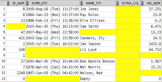
The Results:

In this, next example, the regular expression will allow you to put a coma within a string if you enclose that string in double-quotes.
/* ===== code ===== */

   WITH /* Extract and Cast CSV Data */
     w_csv  as
       ( select  '        ,        ,        ,        '                          x from dual union all
         select  '    8  , 37.251  , "Joe Jones"   , "2009-08-18 13:27:33" '      from dual union all
         select  '   ""  ,  6.471  ,  Sam Smith    , "2010-12-30 16:13:39" '      from dual union all
         select  '   10  ,  0      ,               ,                       '      from dual union all
         select  '   19  , "0.25"  ,  Bob Benson   , " 2003-10-24 23:59:01 " '    from dual union all
         select  '  "47" , 13.23   ,  ","          ,  2007-05-02 22:58:02  '      from dual union all
         select  '  106  , 44.732  ,  "Liz Loyd"   , ""                    '      from dual union all
         select  ' 2249  ,   ""    , "Nelson, Ned"  ,  1997-06-05 04:42:26  '     from dual union all
         select  '" 32154 ",0.001,"Fizwig, Ray, M","1913-02-04 18:01:00"'         from dual union all
         select  '"","42.1234",Sam B Smith,"2010-12-30 16:13:39"'                 from dual union all
         select  '"  12  ",2.4,"",2007-05-02 22:58:02'                            from dual union all
         select  '98,".9732","Jan James,",""'                                     from dual union all
         select  ',,,'                                                            from dual
       )
   , w_elements  as
       ( select  regexp_replace(x,'^ *(".*"|[^,]*) *, *(".*"|[^,]*) *, *(".*"|[^,]*) *, *(".*"|[^,]*) *$','\1')  as c1
              ,  regexp_replace(x,'^ *(".*"|[^,]*) *, *(".*"|[^,]*) *, *(".*"|[^,]*) *, *(".*"|[^,]*) *$','\2')  as c2
              ,  regexp_replace(x,'^ *(".*"|[^,]*) *, *(".*"|[^,]*) *, *(".*"|[^,]*) *, *(".*"|[^,]*) *$','\3')  as c3
              ,  regexp_replace(x,'^ *(".*"|[^,]*) *, *(".*"|[^,]*) *, *(".*"|[^,]*) *, *(".*"|[^,]*) *$','\4')  as c4
           from  w_csv
       )
   , w_data  as
       ( select  to_number(trim('"' from trim(c1)))  as id
              ,  to_number(trim('"' from trim(c2)))  as val
              ,    to_char(trim('"' from trim(c3)))  as nam
              ,    to_date(trim('"' from trim(c4)), 'YYYY-MM-DD HH24:MI:SS')  as dts
           from  w_elements
       )
   SELECT  *
     from  w_data ;
The Results:

Here is an explanation of the two regular expressions used above in the "REGEXP_REPLACE" function.
Note that in these explanations a space is shown as an underscore (_).
In the query's code, the space is a normal space character.

Regular Expression:  '^(.*),(.*),(.*)$'

a)  ^       The string begins,  followed by ...
b)  (       an open parenthesis (the start of a column's value),  followed by ...
c)  .*      zero or more (*) characters of anything (.)
d)  )       a closing parenthesis (the end of a column's value),  followed by ...
              (Note: the above {b through d} is repeated, seperated by commas, for each column of CSV data.)
e)  ,       a comma (,) if there are more columns,  followed by ...
f)  $       the end of the string ($).


Regular Expression:  '^_*(".*"|[^,]*)_*,_*(".*"|[^,]*)_*,_*(".*"|[^,]*)_*$'

a)  ^       The string begins,  followed by ...
b)  _*      zero or more (*) spaces (_),  followed by ...
c)  (       an open parenthesis (the start of a column's value),  followed by ...
d)  ".*"    zero or more (*) characters of anything (.) enclosed by quotes (")
e)  |       OR
f)  [^,]*   zero or more (*) characters of anything except a comma ([^,]),  followed by ...
g)  )       a closing parenthesis (the end of a column's value),  followed by ...
h)  _*      zero or more (*) spaces (_),  followed by ...
              (Note: the above {b through h} is repeated, seperated by commas, for each column of CSV data.)
i)  ,       a comma (,) if there are more columns,  followed by ...
j)  $       the end of the string ($).